AND8327/D
Once the network analyzer data has been exported to
Excel, we compute the real and the imaginary parts of the
fast lane loop vector:
(eq. 17)
VFB + (x1 ) x2) ) jꢁ(y1 ) y2) + X ) jꢁY
Finally, we extract the final loop gain and phase by
entering Equations 8 and 9 in Excel:
p
ń20
x2 + 10A
y2 + 10A
cosǒö
Ǔ
2
(eq. 15)
(eq. 18)
Loopgain + 20 * LOG(SQRT(X ƞ 2 ) Y ƞ 2);10)
2 180
(eq. 19)
Loopphase + DEGREES(ATAN(YńX))
p
ń20
sinǒö
Ǔ
2
(eq. 16)
2 180
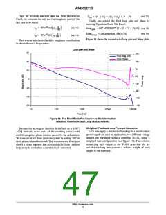
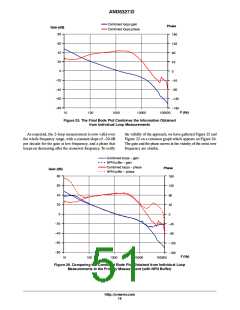
Figure18 shows the reconstructed loop gain and phase plots.
Then we can sum the real and the imaginary contributions
to obtain the total loop vector:
Loop gain and phase
60
40
170
Final Mag (dB)
Final Phase
120
70
20
20
0
-30
-80
-130
-180
-20
-40
-60
10
100
1000
10000
100000
Freq (Hz)
Figure 18. The Final Bode Plot Combines the Information
Obtained from Individual Loop Measurements
Weighted Feedback on a Forward Converter
Because the arctangent function is defined on a ]-90°;
+90°[ interval, some parts of the resulting curve could
exhibit a negative phase rotation caused by the calculation.
We have corrected these particular points by adding 180° to
their phase calculation result. The reconstructed Bode plot
shows a clean response and does not differ from classical
loop analysis carried on a current-mode converter.
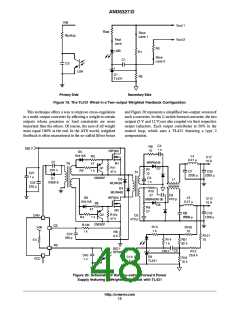
Let's now apply a similar methodology to a multi-output
power supply: in such an application, two different voltage
outputs are regulated using a common TL431, using a
weighted sum configuration (see Figure 19). The resistors
connecting each output to the TL431 reference pin are
calculated taking into account a relative weight of each
output in the feedback.
http://onsemi.com
11

 ETC [ ETC ]