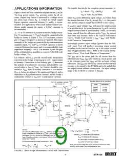
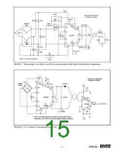
When using linearity correction, care should be taken to
insure that the sensor’s output common-mode voltage re-
mains within the XTR106’s allowable input range of 1.1V to
3.5V. Equation 6 in Figure 3 can be used to calculate the
XTR106’s new excitation voltage. The common-mode volt-
age of the bridge output is simply half this value if no
common-mode resistor is used (refer to the example in
Figure 3). Exceeding the common-mode range may yield
unpredicatable results.
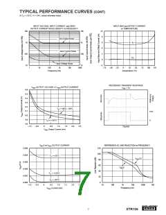
UNDER-SCALE CURRENT
The total current being drawn from the VREF and VREG
voltage sources, as well as temperature, affect the XTR106’s
under-scale current value (see the Typical Performance
Curve, “Under-Scale Current vs IREF + IREG). This should be
considered when choosing the bridge resistance and excita-
tion voltage, especially for transducers operating over a
wide temperature range (see the Typical Performance Curve,
“Under-Scale Current vs Temperature”).
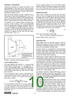
For high precision applications (errors < 1%), a two-step
calibration process can be employed. First, the nonlinearity
of the sensor bridge is measured with the initial gain resistor
and RLIN = 0 (RLIN pin connected directly to VREG). Using
the resulting sensor nonlinearity, B, values for RG and RLIN
are calculated using Equations 4 and 5 from Figure 3. A
second calibration measurement is then taken to adjust RG to
account for the offsets and mismatches in the linearization.
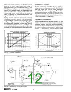
LOW IMPEDANCE BRIDGES
The XTR106’s two available excitation voltages (2.5V and
5V) allow the use of a wide variety of bridge values. Bridge
impedances as low as 1kΩ can be used without any addi-
tional circuitry. Lower impedance bridges can be used with
the XTR106 by adding a series resistance to limit excitation
current to ≤ 2.5mA (Figure 5). Resistance should be added
BRIDGE TRANSDUCER TRANSFER FUNCTION
WITH PARABOLIC NONLINEARITY
10
NONLINEARITY vs STIMULUS
3
9
8
2
Positive Nonlinearity
Positive Nonlinearity
7
B = +0.025
6
B = +0.025
1
5
0
4
B = –0.019
Negative Nonlinearity
–1
3
2
1
0
Linear Response
–2
Negative Nonlinearity
B = –0.019
–3
0
0.1 0.2 0.3 0.4 0.5 0.6 0.7 0.8 0.9
Normalized Stimulus
1
0
0.1 0.2 0.3 0.4 0.5 0.6 0.7 0.8 0.9
Normalized Stimulus
1
FIGURE 4. Parabolic Nonlinearity.
700µA at 5V
VREF5
ITOTAL = 0.7mA + 1.6mA ≤ 2.5mA
VREF2.5
VREG
I
REG ≈ 1.6mA
3.4kΩ
14
13
RLIN
11
1N4148
1
1kΩ
5
4
1/2
OPA2277
V+
10
IN
5V
V+
RG
10kΩ
350Ω
RG
125Ω
9
B
XTR106
0.01µF
412Ω
3
10kΩ
E
RG
V–
8
Lin
Polarity
IO
7
IN
3.4kΩ
2
IRET
1/2
12
OPA2277
6
IO = 4-20mA
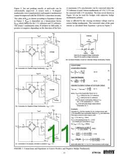
Shown connected to correct positive
bridge nonlinearity. For negative bridge
nonlinearity, see Figure 3b.
Bridge excitation
voltage = 0.245V
Approx. x50
amplifier
FIGURE 5. 350Ω Bridge with x50 Preamplifier.
®
12
XTR106

 BB [ BURR-BROWN CORPORATION ]