The plot for equation (7) is shown in
Figure 5A.3.
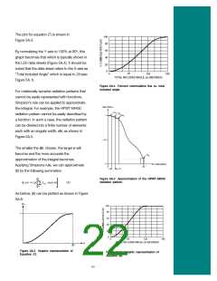
By normalizing the Y-axis to 100% at 90°, this
graph becomes that which is typically shown in
the LED data sheets (Figure 5A.4). It should be
noted that the data sheet refers to the X-axis as
“Total Included Angle” which is equal to 2q (see
Figure 5A.1).
Figure 5A.4 Percent cummulative flux vs. total
included angle.
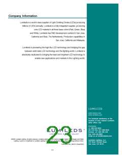
For rotationally symetric radiation patterns that
cannot be easily represented with functions,
Simpson’s rule can be applied to approximate
the integral. For example, the HPWT-MH00
radiation pattern cannot be easily described by
a function. In such a case, the radiation pattern
can be divided into a finite number of elements
each with an angular width, dq, as shown in
Figure 5A.5.
The smaller the dq chosen, the larger n will
become and the more accurate the
approximation of the integral becomes.
Applying Simpsons rule, we can approximate
(6) by the following summation
Figure 5A.5 Approximation of the HPWT-MH00
radiation pattern.
As before, (8) can be plotted as shown in Figure
5A.6.
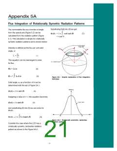
Figure 5A.3 Graphic representation of
Equation (7).
Figure 5A.6 Graphic representation of
equation (8).
22

 LUMILEDS [ LUMILEDS LIGHTING COMPANY ]