AD8307
voltage. T he use of dBV (decibels with respect to 1 V rms) would
be more precise, though still incomplete, since waveform is
involved, too. Since most users think about and specify RF
signals in terms of power—even more specifically, in dBm re 50 Ω
—we will use this convention in specifying the performance of
the AD8307.
in the case of the AD8307, VY is traceable to an on-chip band-
gap reference, while VX is derived from the thermal voltage kT /q
and later temperature-corrected.
Let the input of an N-cell cascade be VIN, and the final output
VOUT . For small signals, the overall gain is simply AN. A six-
stage system in which A = 5 (14 dB) has an overall gain of
15,625 (84 dB). T he importance of a very high small-signal gain
in implementing the logarithmic function has been noted; how-
ever, this parameter is of only incidental interest in the design of
log amps.
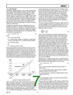
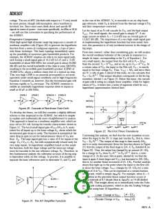
P r ogr essive Com pr ession
Most high speed high dynamic range log amps use a cascade of
nonlinear amplifier cells (Figure 20) to generate the logarithmic
function from a series of contiguous segments, a type of piece-
wise-linear technique. T his basic topology immediately opens
up the possibility of enormous gain-bandwidth products. For
example, the AD8307 employs six cells in its main signal path,
each having a small-signal gain of 14.3 dB (×5.2) and a –3 dB
bandwidth of about 900 MHz; the overall gain is about 20,000
(86 dB) and the overall bandwidth of the chain is some 500 MHz,
resulting in the incredible gain-bandwidth product (GBW) of
10,000 GH z, about a million times that of a typical op amp.
T his very high GBW is an essential prerequisite to accurate
operation under small-signal conditions and at high frequencies.
Equation 2 reminds us, however, that the incremental gain will
decrease rapidly as VIN increases. T he AD8307 continues to
exhibit an essentially logarithmic response down to inputs as
small as 50 µV at 500 MHz.
From here onward, rather than considering gain, we will analyze
the overall nonlinear behavior of the cascade in response to a
simple dc input, corresponding to the VIN of Equation 1. For
very small inputs, the output from the first cell is V1 = AVIN
;
from the second, V2 = A2 VIN, and so on, up to VN = AN VIN. At
a certain value of VIN, the input to the Nth cell, VN–1, is exactly
equal to the knee voltage EK. T hus, VOUT = AEK and since there
are N–1 cells of gain A ahead of this node, we can calculate that
VIN = EK /AN–1. T his unique situation corresponds to the lin-log
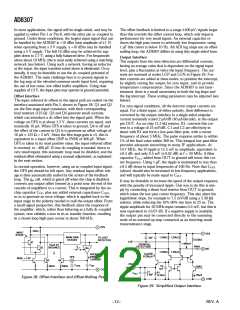
transition, labeled 1 on Figure 22. Below this input, the cascade
of gain cells is acting as a simple linear amplifier, while for higher
values of VIN, it enters into a series of segments which lie on a
logarithmic approximation (dotted line).
STAGE 1
STAGE 2
STAGE N –1
STAGE N
V
OUT
V
(4A-3) E
(3A-2) E
(2A-1) E
AE
V
A
A
A
A
X
W
K
K
K
Figure 20. Cascade of Nonlinear Gain Cells
(A-1) E
K
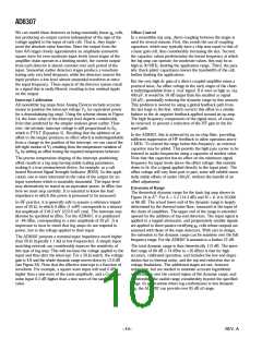
T o develop the theory, we will first consider a slightly different
scheme to that employed in the AD8307, but which is simpler
to explain and mathematically more straightforward to analyze.
T his approach is based on a nonlinear amplifier unit, which we
may call an A/1 cell, having the transfer characteristic shown in
Figure 21. T he local small-signal gain ∂VOUT /∂VIN is A, main-
tained for all inputs up to the knee voltage EK, above which the
incremental gain drops to unity. The function is symmetrical: the
same drop in gain occurs for instantaneous values of VIN less
than –EK. T he large-signal gain has a value of A for inputs in the
range –EK ≤ VIN ≤ +EK, but falls asymptotically toward unity for
very large inputs. In logarithmic amplifiers based on this ampli-
fier function, both the slope voltage and the intercept voltage
must be traceable to the one reference voltage, EK. T herefore, in
this fundamental analysis, the calibration accuracy of the log amp
is dependent solely on this voltage. In practice, it is possible to
separate the basic references used to determine VY and VX and
RATIO
OF A
K
LOG V
IN
0
N–1
N–2
N–3
N–4
/A
E
/A
E
/A
E
/A
E
K
K
K
K
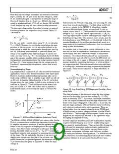
Figure 22. The First Three Transitions
Continuing this analysis, we find that the next transition occurs
when the input to the (N–1) stage just reaches EK; that is, when
VIN = EK /AN–2. T he output of this stage is then exactly AEK,
and it is easily demonstrated (from the function shown in Figure
21) that the output of the final stage is (2A–1) EK (labeled ➁ on
Figure 22). Thus, the output has changed by an amount (A–1)EK
for a change in VIN from EK /AN–1 to EK /AN–2, that is, a ratio
change of A. At the next critical point, labeled ➂, we find the
input is again A times larger and VOUT has increased to (3A–2)EK,
that is, by another linear increment of (A–1)EK. Further analysis
shows that right up to the point where the input to the first cell
is above the knee voltage, VOUT changes by (A–1)EK for a ratio
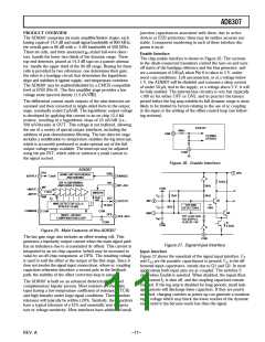
change of A in VIN. T his can be expressed as a certain fraction
of a decade, which is simply log10(A). For example, when A = 5
a transition in the piecewise linear output function occurs at
regular intervals of 0.7 decade (that is, log10(A), or 14 dB divided
by 20 dB). T his insight allows us to immediately write the Volts
per Decade scaling parameter, which is also the Scaling Voltage
VY, when using base-10 logarithms, as:
AE
K
SLOPE = 1
A/1
SLOPE = A
0
E
INPUT
K
A −1 EK
(
=
)
(
Linear Change in VOUT
Decades Change in VIN
VY
=
(4)
log10
A
)
Figure 21. The A/1 Am plifier Function
REV. A
–8–

 ADI [ ADI ]